Defines a prior distribution/probability density function for the average effect size \(d\) or for the heterogeneity of effect sizes \(\tau\).
prior(
  family,
  param,
  lower,
  upper,
  label = "d",
  rel.tol = .Machine$double.eps^0.5
)
Arguments
- family
a character value defining the distribution family.
- param
numeric parameters for the distribution. See details for the definition of the parameters of each family.
- lower
lower boundary for truncatation of prior density. If
family="beta", the interval[0,1]is rescaled to the interval[lower,upper]. Must be specified iffamily = "custom".- upper
See
lower.- label
optional: parameter label.
- rel.tol
relative tolerance used for integrating the density of
family="custom".
Value
an object of the class prior: a density function with the arguments
x (parameter values) and log (whether to return density or log-density).
Details
The following prior distributions are currently implemented:
"norm": Normal distribution withparam = c(mean, sd)(seeNormal)."t": Student's t-distribution withparam = c(location, scale, nu)wherenuare the degrees of freedom (seedist.Student.t)."cauchy": Cauchy distribution withparam = c(location, scale). The Cauchy distribution is a special case of the t-distribution with degrees of freedomnu=1."gamma": Gamma distribution withparam = c(shape, rate)with rate parameter equal to the inverse scale (seeGammaDist)."invgamma": Inverse gamma distribution withparam = c(shape, scale)(seedist.Inverse.Gamma)."beta": (Scaled) beta distribution withparam = c(shape1, shape2)(seeBeta)."custom": User-specified prior density function defined byparam(see examples; the density must be nonnegative and vectorized, but is normalized internally). Integration is performed from (-Inf, Inf), which requires that the function returns zeros (and not NAs) for values not in the support of the distribution.
Examples
### Half-Normal Distribution
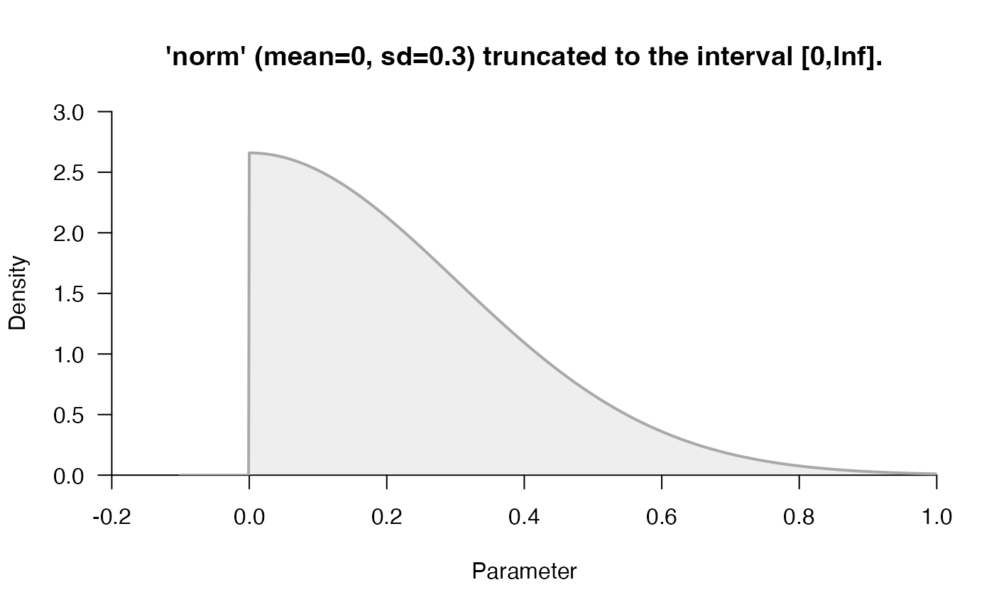
p1 <- prior("norm", c(mean = 0, sd = .3), lower = 0)
p1
#> Prior density function (class='prior'): 'norm' (mean=0, sd=0.3) truncated to the interval [0,Inf].
p1(c(-1, 1, 3))
#> [1] 0.000000e+00 1.028186e-02 5.129732e-22
plot(p1, -.1, 1)


### Half-Cauchy Distribution
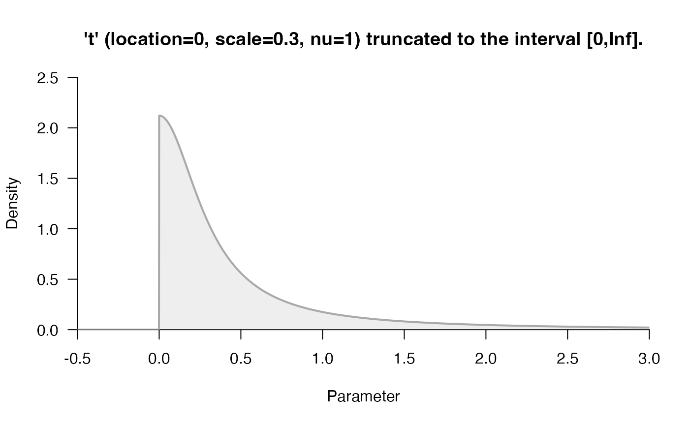
p2 <- prior("cauchy", c(location = 0, scale = .3), lower = 0)
plot(p2, -.5, 3)


### Custom Prior Distribution
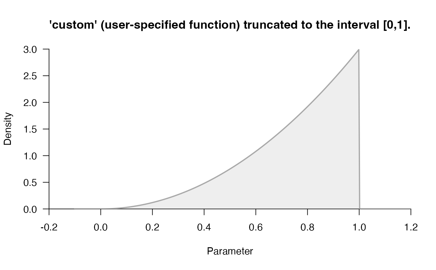
p3 <- prior("custom", function(x) x^2, 0, 1)
plot(p3, -.1, 1.2)
