metaBMA: Bayesian Model Averaging for Random- and Fixed-Effects Meta-Analysis
Daniel W. Heck
2025-07-22
Source:vignettes/metaBMA.Rmd
metaBMA.RmdOverview
Fixed-effects meta-analyses assume that the effect size is identical in all studies. In contrast, random-effects meta-analyses assume that effects vary according to a normal distribution with mean and standard deviation . Both models can be compared in a Bayesian framework by assuming specific prior distribution for and . Given the posterior model probabilities, the evidence for or against an effect (i.e., whether ) and the evidence for or against random effects can be evaluated (i.e., whether ). By using Bayesian model averaging (i.e., inclusion Bayes factors), both types of tests can be performed by marginalizing over the other question. Most importantly, this allows to test whether an effect exists while accounting for uncertainty whether study heterogeneity exists or not.
Defining and Plotting Priors
To fit a meta-analysis model, prior distributions on the average
effect
and the heterogeneity
are required. The package metaBMA leaves the user the
freedom to choose from several predefined distributions or even define
an owen prior density function. The function prior
facilitates the construction and visual inspection of prior
distributions to check whether they meet the prior knowledge about the
field of interest.
## Loading required package: Rcpp## This is metaBMA version 0.6.9## - Default priors were changed in version 0.6.6.## - Since default priors may change again, it is safest to specify priors (even when using the defaults).
# load data set
data(towels)

# Half-normal (truncated to > 0)
p1 <- prior("norm", c(mean=0, sd=.3), lower = 0)
p1
## Prior density function (class='prior'): 'norm' (mean=0, sd=0.3) truncated to the interval [0,Inf].
p1(1:3)## [1] 1.028186e-02 5.940600e-10 5.129732e-22
plot(p1)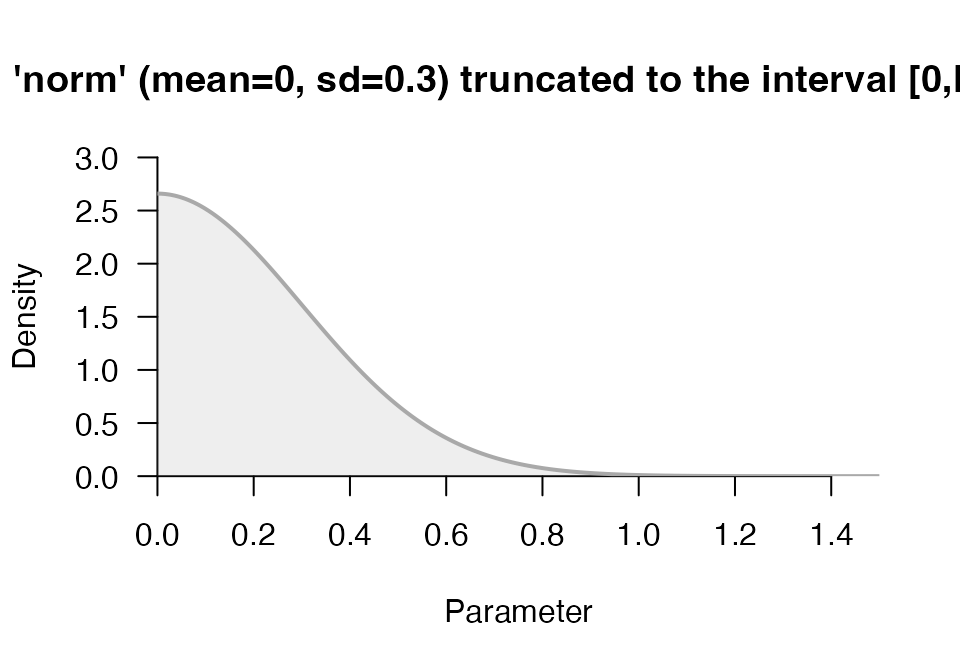
# custom prior
p1 <- prior("custom", function(x) x^3-2*x+3, lower = 0, upper = 1)
plot(p1, -.5, 1.5)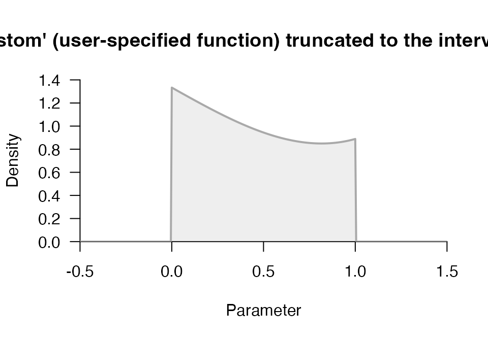
Bayesian Meta-Analysis
The functions meta_fixed() and
meta_random() fit Bayesian meta-analysis models. The
model-specific posteriors for
can then be averaged by bma() and inclusion Bayes factors
be computed by inclusion().
The fixed-effects meta-analysis assumes that the effect size is identical across studies. This model requires only one prior distribution for the overall effect :
# Fixed-effects
progres <- capture.output(  # suppress Stan progress for vignette
  mf <- meta_fixed(logOR, SE, study, towels,
                   d = prior("norm", c(mean=0, sd=.3), lower=0))
)
mf
## ### Bayesian Fixed-Effects Meta-Analysis ###
## Prior on d: 'norm' (mean=0, sd=0.3) truncated to the interval [0,Inf].
##
## # Bayes factors:
## (denominator)
## (numerator) fixed_H0 fixed_H1
## fixed_H0 1.0 0.0419
## fixed_H1 23.9 1.0000
##
## # Posterior summary statistics of fixed-effects model:
## mean sd 2.5% 50% 97.5% hpd95_lower hpd95_upper n_eff Rhat
## d 0.212 0.075 0.066 0.212 0.361 0.062 0.358 NA NA
# plot posterior distribution
plot_posterior(mf)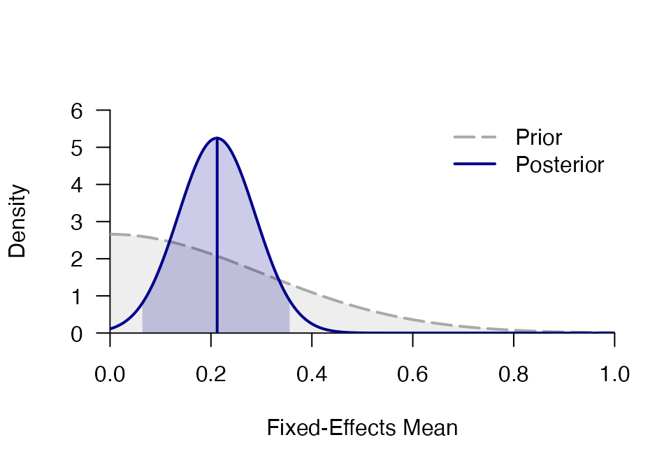
In contrast, the random-effects meta-analysis assumes that the effect size varies across studies. Specifically, it is assumed that study effect sizes follow a normal distribution with mean and standard deviation . This model requires two prior distributions for both parameters:
# Random-effects
progres <- capture.output(  # suppress Stan progress for vignette
  mr <- meta_random(logOR, SE, study, towels,
                    d = prior("norm", c(mean=0, sd=.3), lower=0),
                    tau = prior("t", c(location=0, scale=.3, nu=1), lower=0),
                    iter = 1500, logml_iter = 2000, rel.tol = .1)
)
mr
## ### Bayesian Random-Effects Meta-Analysis ###
## Prior on d: 'norm' (mean=0, sd=0.3) truncated to the interval [0,Inf].
## Prior on tau: 't' (location=0, scale=0.3, nu=1) truncated to the interval [0,Inf].
##
## # Bayes factors:
## (denominator)
## (numerator) random_H0 random_H1
## random_H0 1.00 0.264
## random_H1 3.78 1.000
##
## # Posterior summary statistics of random-effects model:
## mean sd 2.5% 50% 97.5% hpd95_lower hpd95_upper n_eff Rhat
## d 0.195 0.089 0.028 0.195 0.371 0.015 0.354 1812.2 1.002
## tau 0.118 0.107 0.004 0.090 0.395 0.000 0.329 1860.4 1.002
# plot posterior distribution
plot_posterior(mr, main = "Average effect size d")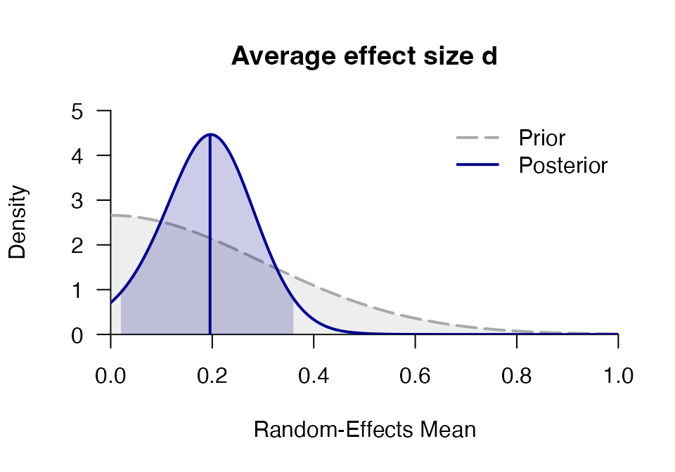
plot_posterior(mr, "tau", main = "Heterogeneity tau")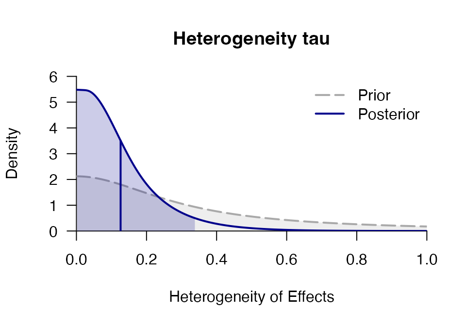
Model-Averaging for Meta-Analysis
The most general functions in metaBMA are
meta_bma() and meta_default(), which fit
random- and fixed-effects models, compute the inclusion Bayes factor for
the presence of an effect and the averaged posterior distribution of the
mean effect
(which accounts for uncertainty regarding study heterogeneity).
mb <- meta_bma(logOR, SE, study, towels,
               d = prior("norm", c(mean=0, sd=.3), lower=0),
               tau = prior("t", c(location=0, scale=.3, nu=1), lower=0),
                    iter = 1500, logml_iter = 2000, rel.tol = .1)
mb
## ### Meta-Analysis with Bayesian Model Averaging ###
## Fixed H0: d = 0
## Fixed H1: d ~ 'norm' (mean=0, sd=0.3) truncated to the interval [0,Inf].
## Random H0: d = 0,
## tau ~ 't' (location=0, scale=0.3, nu=1) truncated to the interval [0,Inf].
## Random H1: d ~ 'norm' (mean=0, sd=0.3) truncated to the interval [0,Inf].
## tau ~ 't' (location=0, scale=0.3, nu=1) truncated to the interval [0,Inf].
##
## # Bayes factors:
## (denominator)
## (numerator) fixed_H0 fixed_H1 random_H0 random_H1
## fixed_H0 1.00 0.0419 0.433 0.114
## fixed_H1 23.87 1.0000 10.330 2.730
## random_H0 2.31 0.0968 1.000 0.264
## random_H1 8.74 0.3663 3.784 1.000
##
## # Bayesian Model Averaging
## Comparison: (fixed_H1 & random_H1) vs. (fixed_H0 & random_H0)
## Inclusion Bayes factor: 9.851
## Inclusion posterior probability: 0.908
##
## # Model posterior probabilities:
## prior posterior logml
## fixed_H0 0.25 0.0278 -5.58
## fixed_H1 0.25 0.6644 -2.40
## random_H0 0.25 0.0643 -4.74
## random_H1 0.25 0.2434 -3.41
##
## # Posterior summary statistics of average effect size:
## mean sd 2.5% 50% 97.5% hpd95_lower hpd95_upper n_eff Rhat
## averaged 0.207 0.078 0.047 0.208 0.365 0.044 0.361 NA NA
## fixed 0.215 0.074 0.068 0.214 0.363 0.060 0.353 953.0 1.005
## random 0.194 0.090 0.026 0.194 0.374 0.011 0.352 1814.1 1.000
plot_posterior(mb, "d", -.1, 1.4)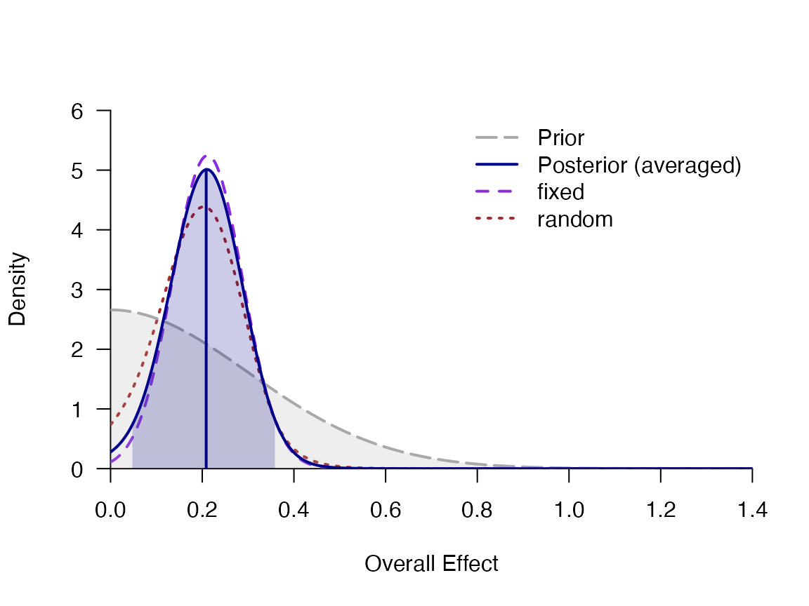
plot_forest(mb)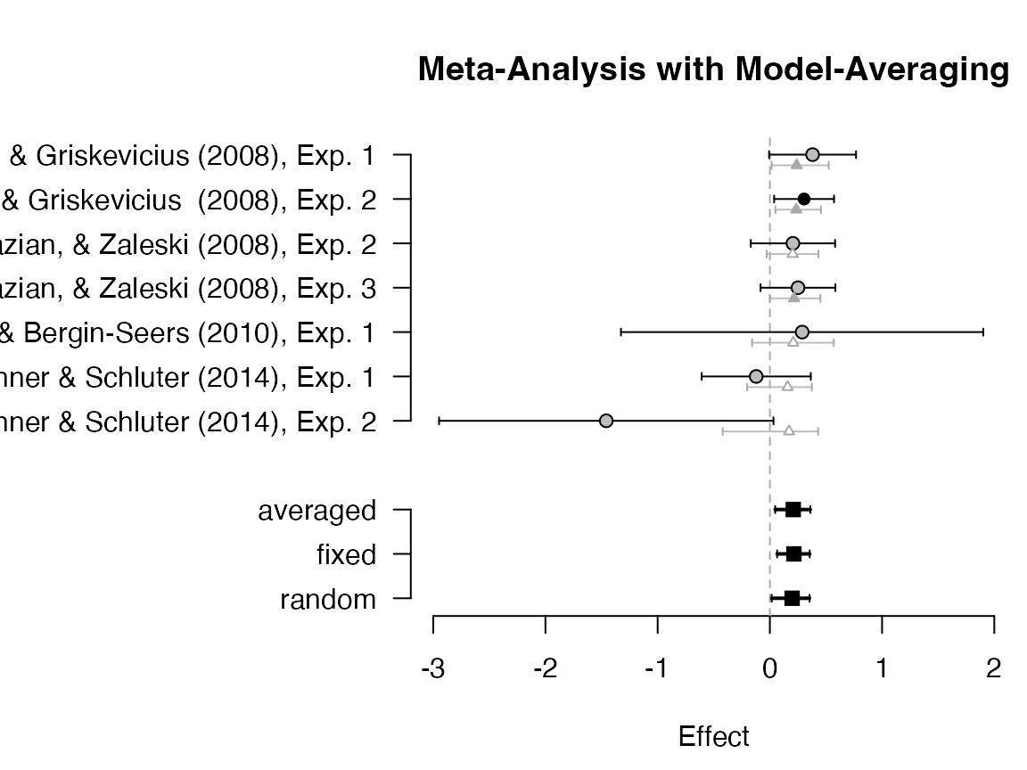
Predicted Bayes Factor for New Study
Often, it is of interest to judge how much additional evidence future
studies can contribute to the present knowledge. Conditional on the
outcome of the model averaging for meta-analysis, the function
predicted_bf() samples new data sets from the posterior and
performs model selection for each replication. Thereby, a distribution
of predicted Bayes factors is obtain that represents the expected
evidence one expects when running a new study. The following example is
not executed since it requires time-intensive computations:
mp <- predicted_bf(mb, SE = .2, sample = 30)
plot(mp)