Bayesian Fixed-Effects Meta-Analysis — meta

Runs a Bayesian meta-analysis assuming that the mean effect $d$ in each study is identical (i.e., a fixed-effects analysis).

meta_fixed(
  y,
  SE,
  labels,
  data,
  d = prior("cauchy", c(location = 0, scale = 0.707)),
  rscale_contin = 1/2,
  rscale_discrete = 0.707,
  centering = TRUE,
  logml = "integrate",
  summarize = "integrate",
  ci = 0.95,
  rel.tol = .Machine$double.eps^0.3,
  silent_stan = TRUE,
  ...
)

Arguments

y: effect size per study. Can be provided as (1) a numeric vector, (2) the quoted or unquoted name of the variable in data, or (3) a formula to include discrete or continuous moderator variables.
SE: standard error of effect size for each study. Can be a numeric vector or the quoted or unquoted name of the variable in data
labels: optional: character values with study labels. Can be a character vector or the quoted or unquoted name of the variable in data
data: data frame containing the variables for effect size y, standard error SE, labels, and moderators per study.
d: prior distribution on the average effect size d. The prior probability density function is defined via prior.
rscale_contin: scale parameter of the JZS prior for the continuous covariates.
rscale_discrete: scale parameter of the JZS prior for discrete moderators.
centering: whether continuous moderators are centered.
logml: how to estimate the log-marginal likelihood: either by numerical integration ("integrate") or by bridge sampling using MCMC/Stan samples ("stan"). To obtain high precision with logml="stan", many MCMC samples are required (e.g., logml_iter=10000, warmup=1000).
summarize: how to estimate parameter summaries (mean, median, SD, etc.): Either by numerical integration (summarize = "integrate") or based on MCMC/Stan samples (summarize = "stan").
ci: probability for the credibility/highest-density intervals.
rel.tol: relative tolerance used for numerical integration using integrate. Use rel.tol=.Machine$double.eps for maximal precision (however, this might be slow).
silent_stan: whether to suppress the Stan progress bar.
...: further arguments passed to rstan::sampling (see stanmodel-method-sampling). Relevant MCMC settings concern the number of warmup samples that are discarded (warmup=500), the total number of iterations per chain (iter=2000), the number of MCMC chains (chains=4), whether multiple cores should be used (cores=4), and control arguments that make the sampling in Stan more robust, for instance: control=list(adapt_delta=.97).

Examples

### Bayesian Fixed-Effects Meta-Analysis (H1: d>0)
data(towels)
mf <- meta_fixed(logOR, SE, study,
  data = towels,
  d = prior("norm", c(mean = 0, sd = .3), lower = 0)
)
mf
#> ### Bayesian Fixed-Effects Meta-Analysis ### 
#>    Prior on d:    'norm' (mean=0, sd=0.3) truncated to the interval [0,Inf]. 
#> 
#> # Bayes factors:
#>            (denominator)
#> (numerator) fixed_H0 fixed_H1
#>    fixed_H0      1.0   0.0419
#>    fixed_H1     23.9   1.0000
#> 
#> # Posterior summary statistics of fixed-effects model:
#>    mean    sd  2.5%   50% 97.5% hpd95_lower hpd95_upper n_eff Rhat
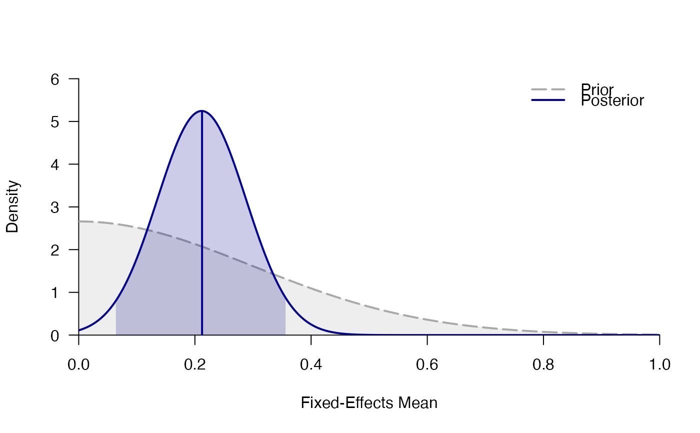
#> d 0.212 0.075 0.066 0.212 0.361       0.062       0.358    NA   NA
plot_posterior(mf)

plot_forest(mf)