Bayesian Model Averaging

Model averaging for different meta-analysis models (e.g., random-effects or fixed-effects with different priors) based on the posterior model probability.

bma(
  meta,
  prior = 1,
  parameter = "d",
  summarize = "integrate",
  ci = 0.95,
  rel.tol = .Machine$double.eps^0.5
)

Arguments

meta

list of meta-analysis models (fitted via meta_random or meta_fixed)

prior

prior probabilities over models (possibly unnormalized). For instance, if the first model is as likely as models 2, 3 and 4 together: prior = c(3,1,1,1). The default is a discrete uniform distribution over models.

parameter

either the mean effect "d" or the heterogeneity "tau" (i.e., the across-study standard deviation of population effect sizes).

summarize

how to estimate parameter summaries (mean, median, SD, etc.): Either by numerical integration (summarize = "integrate") or based on MCMC/Stan samples (summarize = "stan").

ci

probability for the credibility/highest-density intervals.

rel.tol

relative tolerance used for numerical integration using integrate. Use rel.tol=.Machine$double.eps for maximal precision (however, this might be slow).

Examples

# \donttest{
# model averaging for fixed and random effects
data(towels)
fixed <- meta_fixed(logOR, SE, study, towels)
random <- meta_random(logOR, SE, study, towels)
#> Warning: There were 1 divergent transitions after warmup. See
#> https://mc-stan.org/misc/warnings.html#divergent-transitions-after-warmup
#> to find out why this is a problem and how to eliminate them.
#> Warning: Examine the pairs() plot to diagnose sampling problems

averaged <- bma(list("fixed" = fixed, "random" = random))
averaged
#> ### Meta-Analysis with Bayesian Model Averaging ###
#>    Fixed H0:  d = 0 
#>    Fixed H1:  d ~ 't' (location=0, scale=0.707, nu=1) with support on the interval [-Inf,Inf]. 
#>    Random H0: d   = 0,   
#>               tau ~  'invgamma' (shape=1, scale=0.15) with support on the interval [0,Inf]. 
#>    Random H1: d   ~ 't' (location=0, scale=0.707, nu=1) with support on the interval [-Inf,Inf]. 
#>               tau ~ 'invgamma' (shape=1, scale=0.15) with support on the interval [0,Inf]. 
#> 
#> # Bayes factors:
#>            (denominator)
#> (numerator) fixed_H0 fixed_H1 random_H0 random_H1
#>   fixed_H0      1.00    0.203     0.372     0.462
#>   fixed_H1      4.92    1.000     1.830     2.277
#>   random_H0     2.69    0.546     1.000     1.244
#>   random_H1     2.16    0.439     0.804     1.000
#> 
#> # Model posterior probabilities:
#>           prior posterior logml
#> fixed_H0   0.25    0.0928 -5.58
#> fixed_H1   0.25    0.4569 -3.98
#> random_H0  0.25    0.2496 -4.59
#> random_H1  0.25    0.2007 -4.81
#> 
#> # Posterior summary statistics of average effect size:
#>           mean    sd   2.5%   50% 97.5% hpd95_lower hpd95_upper  n_eff Rhat
#> averaged 0.214 0.089  0.034 0.216 0.380       0.040       0.384     NA   NA
#> fixed    0.221 0.078  0.068 0.221 0.375       0.066       0.373     NA   NA
#> random   0.197 0.106 -0.027 0.200 0.393      -0.012       0.404 5290.7    1
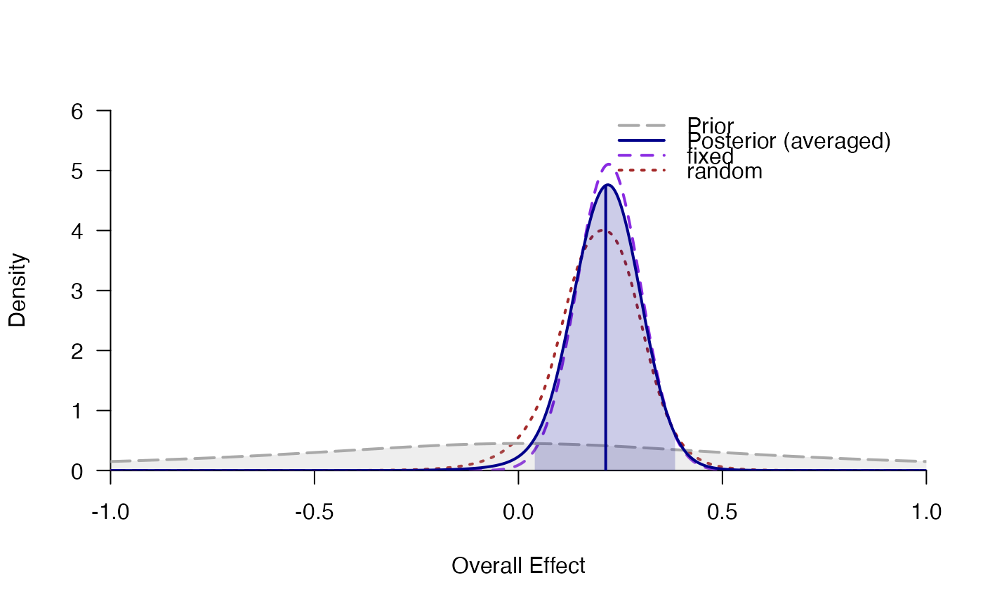
plot_posterior(averaged)

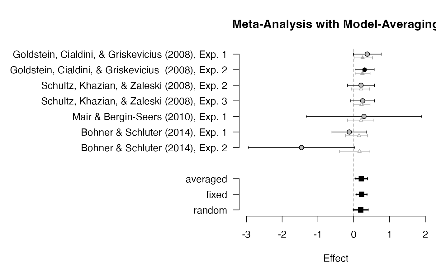
plot_forest(averaged, mar = c(4.5, 20, 4, .3))

# }