Model Averaging for Meta-Analysis

Fits random- and fixed-effects meta-analyses and performs Bayesian model averaging for H1 (d != 0) vs. H0 (d = 0).

meta_bma(
  y,
  SE,
  labels,
  data,
  d = prior("cauchy", c(location = 0, scale = 0.707)),
  tau = prior("invgamma", c(shape = 1, scale = 0.15)),
  rscale_contin = 0.5,
  rscale_discrete = 0.707,
  centering = TRUE,
  prior = c(1, 1, 1, 1),
  logml = "integrate",
  summarize = "stan",
  ci = 0.95,
  rel.tol = .Machine$double.eps^0.3,
  logml_iter = 5000,
  silent_stan = TRUE,
  ...
)

Arguments

y: effect size per study. Can be provided as (1) a numeric vector, (2) the quoted or unquoted name of the variable in data, or (3) a formula to include discrete or continuous moderator variables.
SE: standard error of effect size for each study. Can be a numeric vector or the quoted or unquoted name of the variable in data
labels: optional: character values with study labels. Can be a character vector or the quoted or unquoted name of the variable in data
data: data frame containing the variables for effect size y, standard error SE, labels, and moderators per study.
d: prior distribution on the average effect size d. The prior probability density function is defined via prior.
tau: prior distribution on the between-study heterogeneity tau (i.e., the standard deviation of the study effect sizes dstudy in a random-effects meta-analysis. A (nonnegative) prior probability density function is defined via prior.
rscale_contin: scale parameter of the JZS prior for the continuous covariates.
rscale_discrete: scale parameter of the JZS prior for discrete moderators.
centering: whether continuous moderators are centered.
prior: prior probabilities over models (possibly unnormalized) in the order c(fixed_H0, fixed_H1, random_H0, random_H1). For instance, if we expect fixed effects to be two times as likely as random effects and H0 and H1 to be equally likely: prior = c(2,2,1,1).
logml: how to estimate the log-marginal likelihood: either by numerical integration ("integrate") or by bridge sampling using MCMC/Stan samples ("stan"). To obtain high precision with logml="stan", many MCMC samples are required (e.g., logml_iter=10000, warmup=1000).
summarize: how to estimate parameter summaries (mean, median, SD, etc.): Either by numerical integration (summarize = "integrate") or based on MCMC/Stan samples (summarize = "stan").
ci: probability for the credibility/highest-density intervals.
rel.tol: relative tolerance used for numerical integration using integrate. Use rel.tol=.Machine$double.eps for maximal precision (however, this might be slow).
logml_iter: number of iterations (per chain) from the posterior distribution of d and tau. The samples are used for computing the marginal likelihood of the random-effects model with bridge sampling (if logml="stan") and for obtaining parameter estimates (if summarize="stan"). Note that the argument iter=2000 controls the number of iterations for estimation of the random-effect parameters per study in random-effects meta-analysis.
silent_stan: whether to suppress the Stan progress bar.
...: further arguments passed to rstan::sampling (see stanmodel-method-sampling). Relevant MCMC settings concern the number of warmup samples that are discarded (warmup=500), the total number of iterations per chain (iter=2000), the number of MCMC chains (chains=4), whether multiple cores should be used (cores=4), and control arguments that make the sampling in Stan more robust, for instance: control=list(adapt_delta=.97).

Details

Bayesian model averaging for four meta-analysis models: Fixed- vs. random-effects and H0 ($d=0$) vs. H1 (e.g., $d>0$). For a primer on Bayesian model-averaged meta-analysis, see Gronau, Heck, Berkhout, Haaf, and Wagenmakers (2020).

By default, the log-marginal likelihood is computed by numerical integration (logml="integrate"). This is relatively fast and gives precise, reproducible results. However, for extreme priors or data (e.g., very small standard errors), numerical integration is not robust and might provide incorrect results. As an alternative, the log-marginal likelihood can be estimated using MCMC/Stan samples and bridge sampling (logml="stan").

To obtain posterior summary statistics for the average effect size d and the heterogeneity parameter tau, one can also choose between numerical integration (summarize="integrate") or MCMC sampling in Stan (summarize="stan"). If any moderators are included in a model, both the marginal likelihood and posterior summary statistics can only be computed using Stan.

References

Gronau, Q. F., Erp, S. V., Heck, D. W., Cesario, J., Jonas, K. J., & Wagenmakers, E.-J. (2017). A Bayesian model-averaged meta-analysis of the power pose effect with informed and default priors: the case of felt power. Comprehensive Results in Social Psychology, 2(1), 123-138. doi:10.1080/23743603.2017.1326760

Gronau, Q. F., Heck, D. W., Berkhout, S. W., Haaf, J. M., & Wagenmakers, E.-J. (2021). A primer on Bayesian model-averaged meta-analysis. Advances in Methods and Practices in Psychological Science, 4(3), 1–19. doi:10.1177/25152459211031256

Berkhout, S. W., Haaf, J. M., Gronau, Q. F., Heck, D. W., & Wagenmakers, E.-J. (2023). A tutorial on Bayesian model-averaged meta-analysis in JASP. Behavior Research Methods.

Examples

# \donttest{
### Bayesian Model-Averaged Meta-Analysis (H1: d>0)
data(towels)
set.seed(123)
mb <- meta_bma(logOR, SE, study, towels,
  d = prior("norm", c(mean = 0, sd = .3), lower = 0),
  tau = prior("invgamma", c(shape = 1, scale = 0.15))
)
mb
#> ### Meta-Analysis with Bayesian Model Averaging ###
#>    Fixed H0:  d = 0 
#>    Fixed H1:  d ~ 'norm' (mean=0, sd=0.3) truncated to the interval [0,Inf]. 
#>    Random H0: d   = 0,   
#>               tau ~  'invgamma' (shape=1, scale=0.15) with support on the interval [0,Inf]. 
#>    Random H1: d   ~ 'norm' (mean=0, sd=0.3) truncated to the interval [0,Inf]. 
#>               tau ~ 'invgamma' (shape=1, scale=0.15) with support on the interval [0,Inf]. 
#> 
#> # Bayes factors:
#>            (denominator)
#> (numerator) fixed_H0 fixed_H1 random_H0 random_H1
#>   fixed_H0      1.00   0.0419     0.372    0.0975
#>   fixed_H1     23.87   1.0000     8.872    2.3259
#>   random_H0     2.69   0.1127     1.000    0.2622
#>   random_H1    10.26   0.4299     3.815    1.0000
#> 
#> # Bayesian Model Averaging
#>   Comparison: (fixed_H1 & random_H1) vs. (fixed_H0 & random_H0)
#>   Inclusion Bayes factor: 9.249 
#>   Inclusion posterior probability: 0.902 
#> 
#> # Model posterior probabilities:
#>           prior posterior logml
#> fixed_H0   0.25    0.0264 -5.58
#> fixed_H1   0.25    0.6311 -2.40
#> random_H0  0.25    0.0711 -4.59
#> random_H1  0.25    0.2713 -3.25
#> 
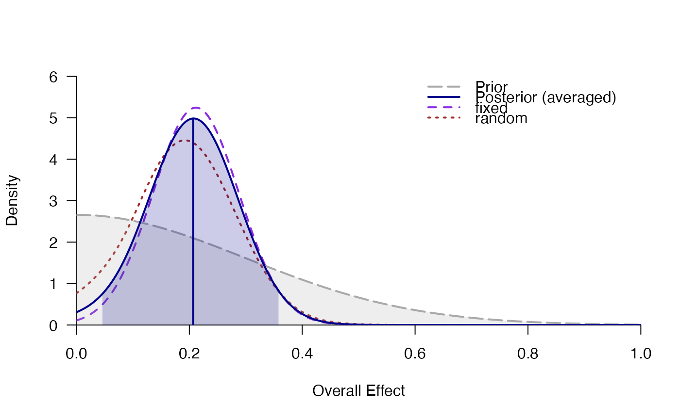
#> # Posterior summary statistics of average effect size:
#>           mean    sd  2.5%   50% 97.5% hpd95_lower hpd95_upper  n_eff  Rhat
#> averaged 0.207 0.080 0.049 0.207 0.364       0.045       0.360     NA    NA
#> fixed    0.215 0.075 0.070 0.215 0.364       0.073       0.365 2095.3 1.001
#> random   0.194 0.088 0.029 0.193 0.370       0.020       0.357 5666.0 1.000
plot_posterior(mb, "d")

# }

Arguments

Details

References

See also

Examples