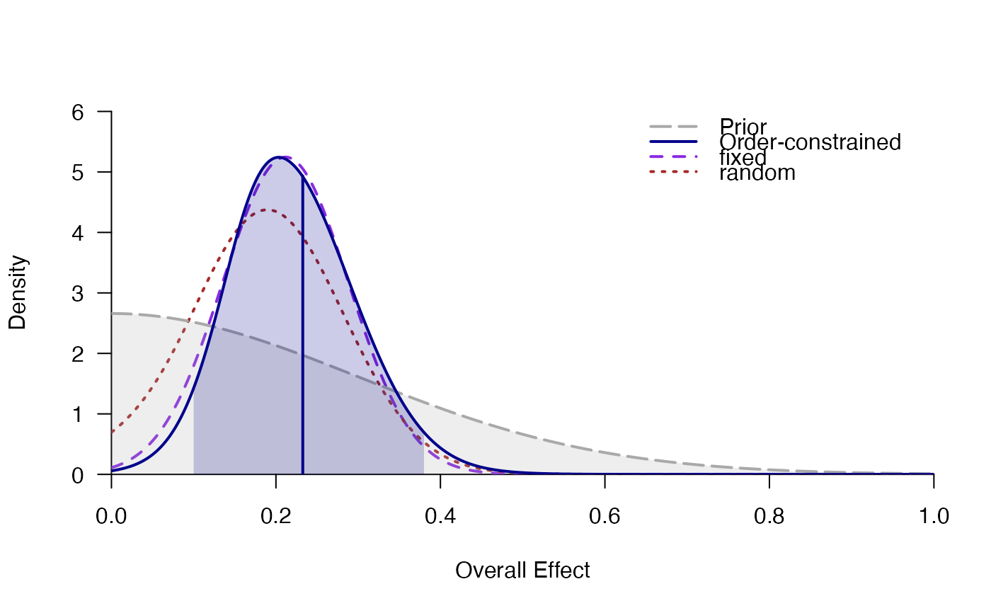
Computes the Bayes factor for the hypothesis that the true study effects in a random-effects meta-analysis are all positive or negative.
meta_ordered(
  y,
  SE,
  labels,
  data,
  d = prior("norm", c(mean = 0, sd = 0.3), lower = 0),
  tau = prior("invgamma", c(shape = 1, scale = 0.15)),
  prior = c(1, 1, 1, 1),
  logml = "integrate",
  summarize = "stan",
  ci = 0.95,
  rel.tol = .Machine$double.eps^0.3,
  logml_iter = 5000,
  iter = 5000,
  silent_stan = TRUE,
  ...
)
Arguments
- y
effect size per study. Can be provided as (1) a numeric vector, (2) the quoted or unquoted name of the variable in
data, or (3) aformulato include discrete or continuous moderator variables.- SE
standard error of effect size for each study. Can be a numeric vector or the quoted or unquoted name of the variable in
data- labels
optional: character values with study labels. Can be a character vector or the quoted or unquoted name of the variable in
data- data
data frame containing the variables for effect size
y, standard errorSE,labels, and moderators per study.- d
priordistribution on the average effect sized. The prior probability density function is defined viaprior.- tau
priordistribution on the between-study heterogeneitytau(i.e., the standard deviation of the study effect sizesdstudyin a random-effects meta-analysis. A (nonnegative) prior probability density function is defined viaprior.- prior
prior probabilities over models (possibly unnormalized) in the order
c(fixed_H0, fixed_H1, ordered_H1, random_H1). Note that the modelrandom_H0is not included in the comparison.- logml
how to estimate the log-marginal likelihood: either by numerical integration (
"integrate") or by bridge sampling using MCMC/Stan samples ("stan"). To obtain high precision withlogml="stan", many MCMC samples are required (e.g.,logml_iter=10000, warmup=1000).- summarize
how to estimate parameter summaries (mean, median, SD, etc.): Either by numerical integration (
summarize = "integrate") or based on MCMC/Stan samples (summarize = "stan").- ci
probability for the credibility/highest-density intervals.
- rel.tol
relative tolerance used for numerical integration using
integrate. Userel.tol=.Machine$double.epsfor maximal precision (however, this might be slow).- logml_iter
number of iterations (per chain) from the posterior distribution of
dandtau. The samples are used for computing the marginal likelihood of the random-effects model with bridge sampling (iflogml="stan") and for obtaining parameter estimates (ifsummarize="stan"). Note that the argumentiter=2000controls the number of iterations for estimation of the random-effect parameters per study in random-effects meta-analysis.- iter
number of MCMC iterations for the random-effects meta-analysis. Needs to be larger than usual to estimate the probability of all random effects being ordered (i.e., positive or negative).
- silent_stan
whether to suppress the Stan progress bar.
- ...
further arguments passed to
rstan::sampling(seestanmodel-method-sampling). Relevant MCMC settings concern the number of warmup samples that are discarded (warmup=500), the total number of iterations per chain (iter=2000), the number of MCMC chains (chains=4), whether multiple cores should be used (cores=4), and control arguments that make the sampling in Stan more robust, for instance:control=list(adapt_delta=.97).
Details
Usually, in random-effects meta-analysis,the study-specific random-effects
are allowed to be both negative or positive even when the prior on the
overall effect size d is truncated to be positive). In contrast, the
function meta_ordered fits and tests a model in which the random
effects are forced to be either all positive or all negative. The direction
of the study-specific random-effects is defined via the prior on the mode of
the truncated normal distribution d. For instance,
d=prior("norm", c(0,.5), lower=0) means that all random-effects are
positive (not just the overall mean effect size).
The posterior summary statistics of the overall effect size in the model
ordered refer to the the average/mean of the study-specific
effect sizes (as implied by the fitted truncated normal distribution) and
not to the location parameter d of the truncated normal
distribution (which is only the mode, not the expected value of a truncated
normal distribution).
The Bayes factor for the order-constrained model is computed using the
encompassing Bayes factor. Since many posterior samples are required for this
approach, the default number of MCMC iterations for meta_ordered is
iter=5000 per chain.
References
Haaf, J. M., & Rouder, J. N. (2018). Some do and some don’t? Accounting for variability of individual difference structures. Psychonomic Bulletin & Review, 26, 772–789. doi:10.3758/s13423-018-1522-x
See also
Examples
# \donttest{
### Bayesian Meta-Analysis with Order Constraints (H1: d>0)
data(towels)
set.seed(123)
mo <- meta_ordered(logOR, SE, study, towels,
  d = prior("norm", c(mean = 0, sd = .3), lower = 0)
)
#> Warning: There were 9 divergent transitions after warmup. See
#> https://mc-stan.org/misc/warnings.html#divergent-transitions-after-warmup
#> to find out why this is a problem and how to eliminate them.
#> Warning: Examine the pairs() plot to diagnose sampling problems
mo
#> ### Bayesian Meta-Analysis with Order Constraints ###
#>    null:    d = 0
#>    fixed:   d ~ 'norm' (mean=0, sd=0.3) truncated to the interval [0,Inf].
#>    ordered: d      ~ 'norm' (mean=0, sd=0.3) truncated to the interval [0,Inf].
#>             tau    ~ 'invgamma' (shape=1, scale=0.15) with support on the interval [0,Inf].
#>             dstudy ~ Normal(d,tau) truncated to [0,Inf]
#>    random:  d      ~ 'norm' (mean=0, sd=0.3) truncated to the interval [0,Inf].
#>             tau    ~ 'invgamma' (shape=1, scale=0.15) with support on the interval [0,Inf].
#>             dstudy ~ Normal(d,tau)
#>
#> # Bayes factors:
#>            (denominator)
#> (numerator) null  fixed ordered random
#>     null     1.0 0.0419  0.0562 0.0975
#>     fixed   23.9 1.0000  1.3408 2.3259
#>     ordered 17.8 0.7458  1.0000 1.7347
#>     random  10.3 0.4299  0.5765 1.0000
#>
#> # Model posterior probabilities:
#>         prior posterior logml
#> null     0.25    0.0189 -5.58
#> fixed    0.25    0.4509 -2.40
#> ordered  0.25    0.3363 -2.70
#> random   0.25    0.1939 -3.25
#>
#> # Posterior summary statistics of average effect size:
#>          mean    sd  2.5%   50% 97.5% hpd95_lower hpd95_upper   n_eff Rhat
#> fixed   0.214 0.076 0.070 0.213 0.363       0.067       0.360  3288.5    1
#> ordered 0.236 0.074 0.106 0.230 0.394       0.094       0.378      NA   NA
#> random  0.194 0.088 0.029 0.194 0.371       0.017       0.352 11378.8    1
plot_posterior(mo)

# }
# }