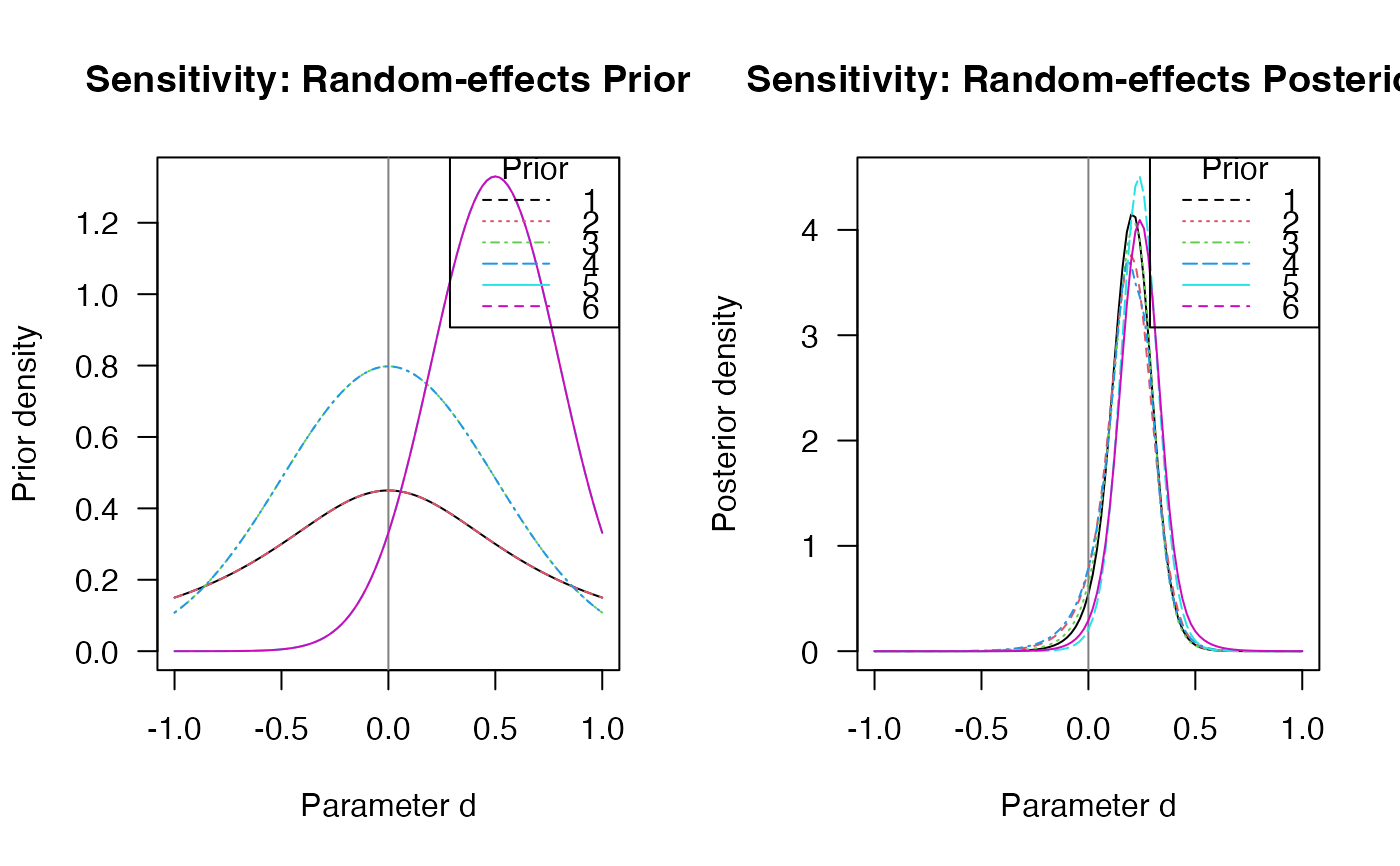
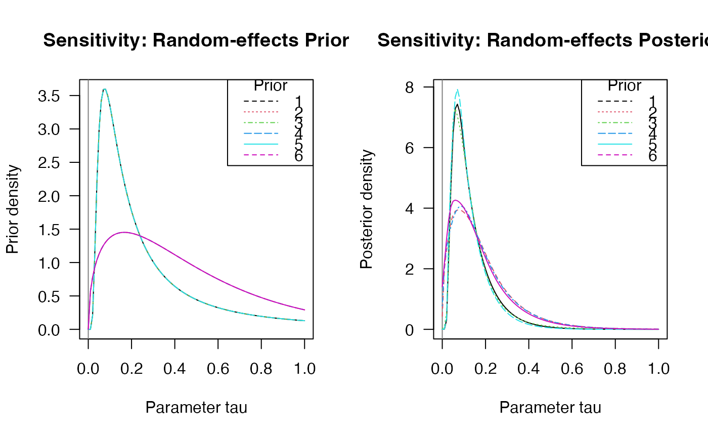
Sensitivity Analysis for Bayesian Meta-Analysis

Sensitivity analysis assuming different prior distributions for the two main parameters of a Bayesian meta-analysis (i.e., the overall effect and the heterogeneity of effect sizes across studies).

meta_sensitivity(
  y,
  SE,
  labels,
  data,
  d_list,
  tau_list,
  analysis = "bma",
  combine_priors = "crossed",
  ...
)

Arguments

y

effect size per study. Can be provided as (1) a numeric vector, (2) the quoted or unquoted name of the variable in data, or (3) a formula to include discrete or continuous moderator variables.

SE

standard error of effect size for each study. Can be a numeric vector or the quoted or unquoted name of the variable in data

labels

optional: character values with study labels. Can be a character vector or the quoted or unquoted name of the variable in data

data

data frame containing the variables for effect size y, standard error SE, labels, and moderators per study.

d_list

a list of prior distributions specified via prior() for the overall effect size (mean) across studies

tau_list

a list of prior distributions specified via prior() for the heterogeneity (SD) of effect sizes across studies

analysis

which type of meta-analysis should be performed for analysis? Can be one of the following:

"fixed" for fixed-effects model, see meta_fixed()
"random" for random-effects model, see meta_random()
"bma" for model averaging, see meta_bma()

combine_priors

either "matched", in which case the analysis includes the matched pairwise combinations of the prior distributions specified in d_list and tau_list, or crossed, in which case the analysis uses all possible pairwise combinations of priors.

...

further arguments passed to the function specified in analysis.

Value

an object of the S3 class meta_sensitivity, that is, a list of fitted meta-analysis models. Results can be printed or plotted using plot.meta_sensitivity().

Examples

# \donttest{
data(towels)
sensitivity <- meta_sensitivity(
  y = logOR, SE = SE, labels = study, data = towels,
  d_list = list(prior("cauchy", c(0, .707)),
                prior("norm", c(0, .5)),
                prior("norm", c(.5, .3))),
  tau_list = list(prior("invgamma", c(1, 0.15), label = "tau"),
                  prior("gamma", c(1.5, 3), label = "tau")),
  analysis = "random",
  combine_priors = "crossed")
#> Warning: There were 1 divergent transitions after warmup. See
#> https://mc-stan.org/misc/warnings.html#divergent-transitions-after-warmup
#> to find out why this is a problem and how to eliminate them.
#> Warning: Examine the pairs() plot to diagnose sampling problems
#> Warning: There were 2 divergent transitions after warmup. See
#> https://mc-stan.org/misc/warnings.html#divergent-transitions-after-warmup
#> to find out why this is a problem and how to eliminate them.
#> Warning: Examine the pairs() plot to diagnose sampling problems
#> Warning: There were 2 divergent transitions after warmup. See
#> https://mc-stan.org/misc/warnings.html#divergent-transitions-after-warmup
#> to find out why this is a problem and how to eliminate them.
#> Warning: Examine the pairs() plot to diagnose sampling problems

print(sensitivity, digits = 2)
#> ### Sensitivity analysis for Bayesian meta-analysis ###
#> 
#> Prior distributions on d (= overall effect size):
#> 
#> [1] "'t' (location=0, scale=0.707, nu=1) with support on the interval [-Inf,Inf]."
#> [2] "'t' (location=0, scale=0.707, nu=1) with support on the interval [-Inf,Inf]."
#> [3] "'norm' (mean=0, sd=0.5) with support on the interval [-Inf,Inf]."            
#> [4] "'norm' (mean=0, sd=0.5) with support on the interval [-Inf,Inf]."            
#> [5] "'norm' (mean=0.5, sd=0.3) with support on the interval [-Inf,Inf]."          
#> [6] "'norm' (mean=0.5, sd=0.3) with support on the interval [-Inf,Inf]."          
#> 
#> Prior distributions on tau (= SD of effect sizes):
#> 
#> [1] "'invgamma' (shape=1, scale=0.15) with support on the interval [0,Inf]."
#> [2] "'gamma' (shape=1.5, rate=3) with support on the interval [0,Inf]."     
#> [3] "'invgamma' (shape=1, scale=0.15) with support on the interval [0,Inf]."
#> [4] "'gamma' (shape=1.5, rate=3) with support on the interval [0,Inf]."     
#> [5] "'invgamma' (shape=1, scale=0.15) with support on the interval [0,Inf]."
#> [6] "'gamma' (shape=1.5, rate=3) with support on the interval [0,Inf]."     
#> 
#> Parameter estimates:
#> 
#>      prior mean    sd   2.5%  50% 97.5% hpd95_lower hpd95_upper n_eff Rhat
#> d1       1 0.20 0.105 -0.026 0.20  0.39    -0.01344        0.40  4873    1
#> d2       2 0.19 0.124 -0.090 0.19  0.41    -0.06496        0.43  3602    1
#> d3       3 0.19 0.109 -0.036 0.20  0.39    -0.02826        0.40  4590    1
#> d4       4 0.18 0.127 -0.111 0.19  0.40    -0.07553        0.43  3511    1
#> d5       5 0.24 0.096  0.045 0.24  0.42     0.03746        0.42  5990    1
#> d6       6 0.24 0.108  0.024 0.24  0.45     0.02630        0.45  4448    1
#> tau1     1 0.13 0.103  0.033 0.11  0.38     0.02041        0.31  2397    1
#> tau2     2 0.18 0.141  0.015 0.14  0.54     0.00158        0.45  3166    1
#> tau3     3 0.14 0.117  0.033 0.11  0.41     0.01776        0.33   722    1
#> tau4     4 0.18 0.145  0.016 0.14  0.56     0.00053        0.46  3046    1
#> tau5     5 0.12 0.087  0.033 0.10  0.36     0.02086        0.29  4611    1
#> tau6     6 0.17 0.134  0.013 0.13  0.52     0.00035        0.43  3461    1
#> 
#> Posterior model probabilities:
#> 
#>        random_H0 random_H1
#> prior1      0.55      0.45
#> prior2      0.63      0.37
#> prior3      0.41      0.59
#> prior4      0.50      0.50
#> prior5      0.38      0.62
#> prior6      0.47      0.53

par(mfrow = c(1,2))
plot(sensitivity, "d", "prior")
#> Prior distributions on d (= overall effect size):
#> 
#> [1] "'t' (location=0, scale=0.707, nu=1) with support on the interval [-Inf,Inf]."
#> [2] "'t' (location=0, scale=0.707, nu=1) with support on the interval [-Inf,Inf]."
#> [3] "'norm' (mean=0, sd=0.5) with support on the interval [-Inf,Inf]."            
#> [4] "'norm' (mean=0, sd=0.5) with support on the interval [-Inf,Inf]."            
#> [5] "'norm' (mean=0.5, sd=0.3) with support on the interval [-Inf,Inf]."          
#> [6] "'norm' (mean=0.5, sd=0.3) with support on the interval [-Inf,Inf]."          
#> 
#> Prior distributions on tau (= SD of effect sizes):
#> 
#> [1] "'invgamma' (shape=1, scale=0.15) with support on the interval [0,Inf]."
#> [2] "'gamma' (shape=1.5, rate=3) with support on the interval [0,Inf]."     
#> [3] "'invgamma' (shape=1, scale=0.15) with support on the interval [0,Inf]."
#> [4] "'gamma' (shape=1.5, rate=3) with support on the interval [0,Inf]."     
#> [5] "'invgamma' (shape=1, scale=0.15) with support on the interval [0,Inf]."
#> [6] "'gamma' (shape=1.5, rate=3) with support on the interval [0,Inf]."     
plot(sensitivity, "d", "posterior")

#> Prior distributions on d (= overall effect size):
#> 
#> [1] "'t' (location=0, scale=0.707, nu=1) with support on the interval [-Inf,Inf]."
#> [2] "'t' (location=0, scale=0.707, nu=1) with support on the interval [-Inf,Inf]."
#> [3] "'norm' (mean=0, sd=0.5) with support on the interval [-Inf,Inf]."            
#> [4] "'norm' (mean=0, sd=0.5) with support on the interval [-Inf,Inf]."            
#> [5] "'norm' (mean=0.5, sd=0.3) with support on the interval [-Inf,Inf]."          
#> [6] "'norm' (mean=0.5, sd=0.3) with support on the interval [-Inf,Inf]."          
#> 
#> Prior distributions on tau (= SD of effect sizes):
#> 
#> [1] "'invgamma' (shape=1, scale=0.15) with support on the interval [0,Inf]."
#> [2] "'gamma' (shape=1.5, rate=3) with support on the interval [0,Inf]."     
#> [3] "'invgamma' (shape=1, scale=0.15) with support on the interval [0,Inf]."
#> [4] "'gamma' (shape=1.5, rate=3) with support on the interval [0,Inf]."     
#> [5] "'invgamma' (shape=1, scale=0.15) with support on the interval [0,Inf]."
#> [6] "'gamma' (shape=1.5, rate=3) with support on the interval [0,Inf]."     

plot(sensitivity, "tau", "prior")
#> Prior distributions on d (= overall effect size):
#> 
#> [1] "'t' (location=0, scale=0.707, nu=1) with support on the interval [-Inf,Inf]."
#> [2] "'t' (location=0, scale=0.707, nu=1) with support on the interval [-Inf,Inf]."
#> [3] "'norm' (mean=0, sd=0.5) with support on the interval [-Inf,Inf]."            
#> [4] "'norm' (mean=0, sd=0.5) with support on the interval [-Inf,Inf]."            
#> [5] "'norm' (mean=0.5, sd=0.3) with support on the interval [-Inf,Inf]."          
#> [6] "'norm' (mean=0.5, sd=0.3) with support on the interval [-Inf,Inf]."          
#> 
#> Prior distributions on tau (= SD of effect sizes):
#> 
#> [1] "'invgamma' (shape=1, scale=0.15) with support on the interval [0,Inf]."
#> [2] "'gamma' (shape=1.5, rate=3) with support on the interval [0,Inf]."     
#> [3] "'invgamma' (shape=1, scale=0.15) with support on the interval [0,Inf]."
#> [4] "'gamma' (shape=1.5, rate=3) with support on the interval [0,Inf]."     
#> [5] "'invgamma' (shape=1, scale=0.15) with support on the interval [0,Inf]."
#> [6] "'gamma' (shape=1.5, rate=3) with support on the interval [0,Inf]."     
plot(sensitivity, "tau", "posterior")

#> Prior distributions on d (= overall effect size):
#> 
#> [1] "'t' (location=0, scale=0.707, nu=1) with support on the interval [-Inf,Inf]."
#> [2] "'t' (location=0, scale=0.707, nu=1) with support on the interval [-Inf,Inf]."
#> [3] "'norm' (mean=0, sd=0.5) with support on the interval [-Inf,Inf]."            
#> [4] "'norm' (mean=0, sd=0.5) with support on the interval [-Inf,Inf]."            
#> [5] "'norm' (mean=0.5, sd=0.3) with support on the interval [-Inf,Inf]."          
#> [6] "'norm' (mean=0.5, sd=0.3) with support on the interval [-Inf,Inf]."          
#> 
#> Prior distributions on tau (= SD of effect sizes):
#> 
#> [1] "'invgamma' (shape=1, scale=0.15) with support on the interval [0,Inf]."
#> [2] "'gamma' (shape=1.5, rate=3) with support on the interval [0,Inf]."     
#> [3] "'invgamma' (shape=1, scale=0.15) with support on the interval [0,Inf]."
#> [4] "'gamma' (shape=1.5, rate=3) with support on the interval [0,Inf]."     
#> [5] "'invgamma' (shape=1, scale=0.15) with support on the interval [0,Inf]."
#> [6] "'gamma' (shape=1.5, rate=3) with support on the interval [0,Inf]."     
# }

Arguments

Value

See also

Examples